Uplevel Big Data Analytics with Graph in Vertica – Part 2: Yes, you can write that in SQL
Uplevel Big Data Analytics with Graph in Vertica – Part 2: Yes, you can write that in SQL
by Walter Maguire, HP
In my prior blog post on graph, I described a very basic form of graph analysis and how one of our customers applied this technique in the HP Vertica big data analytics database to significantly improve their business. What I’ll do in this entry is review how a common graph algorithm – single-source shortest path – is set up and executed in Vertica. I’ll also provide performance results comparing the performance of shortest path between Vertica and two popular graph engines.
“When you come to a fork in the road, take it.” –Yogi Berra
One of the more commonly used graph algorithms is called “Single-source, shortest path.” This algorithm aims to calculate the shortest path from a given starting node to where the path ends in the graph. An easy way to think of this is to imagine the starting node as a pizza shop. The edges in this graph would be streets, and the other nodes are homes where people might want pizza. The shortest path algorithm would compute the path from the pizza shop to each of the homes so we can identify which is the shortest. This can really come in handy when you’ve got pizza to deliver!
In social media, shortest path is a fundamental computation – the sort of thing we do to enrich the graph so we can derive powerful insights. If we take the example of Twitter, a node might be a person, and the edge is the propagation of a tweet – a retweet perhaps. Once we compute shortest path we can understand things such as:
What is the shortest path a tweet took from one person to another? Once we’ve identified the path length from a given starting point, it’s easy enough to filter down to just the paths which end at a given end point.
How quickly does an idea propagate? Now we can test the old saying that “bad news travels fast.” This might be highly useful for a business monitoring its brand – if something negative happens and we know how quickly those ideas can propagate across Twitter, we can think about ways to respond quickly enough to make a difference.
To do this in Vertica is very straightforward. The schema consists of two tables: edge and node. Edge contains the to- and from- node ids reflecting the relationship between each pair of connected nodes, and possibly other information pertaining to the edge such as weight. Node contains the node ids and possibly information about the node. In our tests, we used a publicly available Twitter dataset where people are nodes (aka vertices) and relationships between people (such as being a follower) define the edges.
Let’s assume that my Twitter follower graph looks like this:
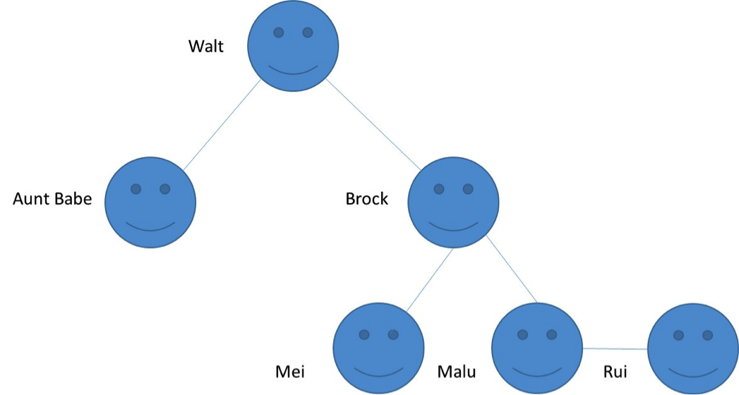
Computing shortest path is an iterative process which starts from a designated spot and traverses the graph until it can’t iterate further. The processing is like this:
- Given a starting node (Walt), check whether that node has any children. This node gets a distance of zero – because aside from a few existential quirks I don’t need to go anywhere to find myself!
- For each of the child nodes (Aunt Babe, Brock), set their distance value to be our numeric representation of “distance” from the starting node. Let’s say we set that value to 1.
- Given each of the child nodes we just evaluated, check whether those nodes have any children.
- For each child node identified in step 3 (Mei, Malu), set their distance value to be the sum of the parent node’s distance value plus the new distance. If distance is “1”, and the parent has a distance of 1, then 1+1=2. The distance value we set for these children is 2.
- Repeat steps 3 and 4 until we find no more nodes with children.
- The final distances we end up with would be as follows:

At this point we have a dataset which indicates all the path distances from a given starting node to the end of each path. So not only can we identify shortest path, we can also identify longest path, average path, median path, etc. We can also apply weights to reflect the fact that some paths may be more (or less) important than others. For example, if an industry analyst picks up one of my tweets and retweets it, this might reflect a shorter “path” because it’s a better outcome for me versus Aunt Babe picking up my tweet and retweeting it just to be nice.
So we could look at this and decide that the shortest path between me and my follower chain ends at Aunt Babe, who has a path value of one. Kind of useful, but there’s a lot more we could learn from this. For example, I may want to find the length of all paths between a Gartner analyst and myself so I can identify the shortest path. In other words, what was the optimal follower path between the analyst and myself? Maybe there are people in that path I want to get to know better in order to gain more mindshare with Gartner. With shortest path, we can ask a wide variety of questions like this. In other words, we can explore the relationships between people (and ideas) at scale, very quickly.
So…what incredibly complex SQL did we have to write for this? Hold on to your hats…
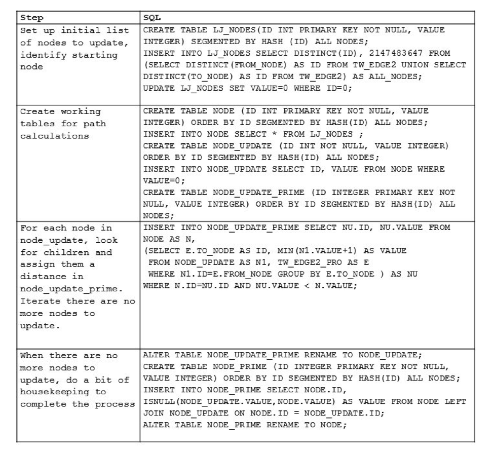
Gosh, that’s complicated. It took me all of twenty minutes to explain it to my twelve-year-old.
The bit of table shuffling you see (renaming tables) is part of a rudimentary optimization technique based on things DBAs have known for decades – that DDL operations are often faster at large scales than DML operations. So if you want to make a bunch of updates go fast, sometimes it’s faster to shove them into a new table with the set of values which *aren’t* being updated, then replace the old table with the new one.
“Okay Walt,” I can hear the skeptical data science type saying, “So you can write it in SQL. That doesn’t mean it’ll ever return a result.”
With anything other than Vertica that might be correct. However, the team ran this SQL analytics test on a Twitter dataset with 41.6 million nodes and 1.4 billion edges. And Vertica outperformed two well-known, dedicated graph engines – Giraph and GraphLab – on the exact same hardware, performing the calculation 8% and 29% faster, respectively.
Why the performance differential?
When we peer into the details observed during the tests, some interesting patterns emerge. First, the both Giraph and GraphLab spent a large amount of time setting up the data for analysis. On the other hand, Vertica was significantly faster in this phase. The graph engines both were very quick when implementing the algorithm, but because Vertica was so much more performant in the load and setup phase they nevertheless took longer overall.
This makes sense when we consider the origin of the graph engines versus Vertica. The graph engines are basically implementations of one or more graph algorithms, whereas Vertica is first and foremost an efficient storage and retrieval engine. If we look at any piece of software as the sum of a set of choices as to where to invest our time, and that these investments yield steady improvements in that domain, the different performance characteristics make perfect sense. If as a developer I want to quickly implement a graph algorithm, I’m not going to spend much time developing efficient storage. That would make no sense. Interestingly, by developing a column-oriented, parallel storage and retrieval engine first, Vertica has set itself up for some very interesting possibilities.
Another implication of the observed performance characteristics is that Vertica can significantly improve performance. For example, during the tests, Vertica was slower during the processing of the shortest path algorithm. This makes sense because we started building Vertica as a database, not a graph engine. But as we choose to invest in improving the efficiency of graph processing, we can make dramatic performance improvements. I’ll discuss some of these possibilities in my next blog post.
So let’s see where we stand on the myths discussed in part 1 of this blog series:
Myth 1: Graph operations are highly iterative and ill-suited to RDBMS technology
Busted! The necessary looping was done with a rudimentary bit of procedural scripting.
Myth 2: Graph operations are too hard to express in SQL
Busted! For those who think thirty or so lines of SQL is too complex, consider hiring some easy to find database talent. It’ll cost you a lot less than the “MPP/graph/machine learning/distributed programming/expert in six programming languages” unicorn you’d need without SQL.
Myth 3: Relational databases aren’t fast/scalable enough to perform graph operations
Busted! With minimal effort, Vertica outperforms two well-known and widely used graph engines. And there are many tweaks we can make to further improve performance.
Well, it seems I’m ahead of schedule, having already busted the three myths identified in part 1. But wait, there’s more! As we look more closely into the benchmark, we observed that there are a number of ways we can further enhance Vertica’s performance at graph. Furthermore, there are certain graph problems which vertex centric graph engines can’t express well, which are trivial in an RDBMS. Finally, there are synergies to be found by doing this in the same engine used for other forms of data analytics. I’ll discuss these topics in future entries.
Next up: “Yes, you can make it go even faster”
——————————————————–
Resources
Graph Analytics using the Vertica Relational Database by Jindal et al.
Get it right the first time with big data analytics by Joy King
Chasing the dream or trying to change the world? Insights and opinion on Hackathons by Sean Hughes
Born in a data-driven world by Joy King
Uplevel Big Data analytics with HP Vertica – Part 1: Graph in a relational database? Seriously? by Walter Maguire