Uplevel Big Data Analytics with Graph in Vertica – Part 3: Yes, you can make it go even faster

Uplevel Big Data Analytics with Graph in Vertica – Part 3: Yes, you can make it go even faster

BY Walter Maguire, HP

So far in this blog series, I’ve discussed the concept of graph analysis and provided an example of how we implemented and benchmarked one common algorithm – single source shortest path – comparing Vertica to several common graph engines. In this post, I’ll discuss the observed performance characteristics in more detail and provide some insights as to how we can further optimize performance of graph analytics in the Vertica engine.

“Time is money” –Ben Franklin

First, let’s recap the observed performance of Vertica and set a baseline for talking about optimization. The team ran this test on a Twitter dataset with 41.6 million nodes and 1.4 billion edges. Vertica outperformed two well-known, dedicated graph engines – Giraph and GraphLab – on the exact same hardware, performing the calculation 8% and 29% faster, respectively.

When we peer into the details observed during the tests, some interesting patterns emerge. Processing fell into two clear phases – setup and retrieval of the data, and processing the graph algorithm. Both Giraph and GraphLab spent a large amount of time setting up the data for analysis. On the other hand, Vertica was significantly faster in this phase. The graph engines both were faster processing the algorithm, but because Vertica was so much more performant in the load and setup phase, they nevertheless took longer overall.

This makes sense when we consider the origin of graph engines versus Vertica. Graph engines are basically implementations of one or more graph algorithms, whereas Vertica is first and foremost an efficient storage and retrieval engine. If we look at any piece of software as the sum of a set of choices as to where to invest our time, and that these investments yield steady improvements in that domain, the different performance characteristics make perfect sense. If, as a developer, I want to quickly implement a graph algorithm, I’m not going to spend much time developing efficient storage. That would make no sense. Interestingly, by developing a column-oriented, parallel storage and retrieval engine first, Vertica has set itself up for some very interesting possibilities. Graph is one of them.

Based on this, two areas emerge as potential targets for performance optimization: 1) fully leveraging the MPP nature of the system, and 2) more efficiently implementing the graph algorithm.

Make it go fast, Part 1: Fully leveraging the MPP architecture

Let’s start with what I call “MPP 101,” so this discussion will make sense. When we reference something like an “MPP database,” what we’re typically referring to is a system which takes a collection of low cost, small systems and makes them behave as a single entity for the purposes of data processing. The power of this is that we can build massive databases out of large collections of relatively low cost systems.

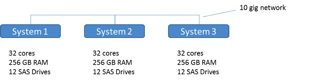
Figure 1 below depicts my simple version of a three-node MPP system.   This consists of three computers – each of which has 32 cores, 256 gigabytes of RAM and 12 SAS hard drives, connected by a 10 gigabyte network. In total, this MPP system has 96 cores, 768 gigabytes of RAM, and 36 SAS hard drives. That’s a lot of I/O, RAM and cores! And it has a 10 gigabyte network. If we double the size of the system by adding three more nodes, now we’ve got 192 cores, over 1.5 terabytes of RAM, and 72 hard drives. Wow! And it still has…a 10 gigabyte interconnect. Hmm.

Location, location, location

The most precious resource in any MPP system is network. While we can deploy massive amounts of processing power, I/O bandwidth and memory, we can’t do the same with network. So one of the most important things we need to do for optimizing performance at scale in an MPP system is to localize the processing as much as possible.

Because an MPP database has to respond as a single database, it has to share information across nodes. For example, if I want to run a query in parallel across all three nodes, but one of the tables used by the query resides on a single node, the system would have to ship that table across the network to the other two nodes for use in the query. If this table is large, or this is done often, it would degrade the overall performance of the system.

So, at a minimum we have to make sure that operations like table joins are localized. This is the first optimization we can do with graph processing. In Vertica, we call the practice of distributing a table across the cluster “segmentation”. By segmenting the tables containing the graph data the same way across the cluster, joins are localized. This significantly improves performance. Moreover, because we reinvented database storage to loosely couple logical schema from physical storage with a structure called a projection, we allow users to create additional projections for a table.

These can be segmented different ways.  This helps us solve a thorny issue with graph data – sometimes we need to join the graph data different ways for different queries. By being able to create additional projections which segment the data differently, we can insure consistent good performance without needing to alter the data model queried by the user. This is a very useful technique our customers have been using for many years.

Parallel versus PARALLEL

While locality of operations such as joins will improve performance, what about leveraging parallelism within a node? That’s got to be a no brainer, right? Wrong! It turns out that MPP systems frequently suffer from the ability to fully parallelize operations within a node. What this means is that when you run a query that distributes activity across the nodes, if you were to look within any one node you might see that perhaps two or three cores were busy and the rest are…idle! What a waste of resources!

This is the difference between a five year old product and a ten year old product. When building any massively parallel system, everybody starts with the first step towards parallelism – distribute activity across nodes. But it takes a mature optimizer which is able to do things like match intra-node parallelism to the characteristics of the query and fully use all the cores on any given node. This is a feature we built into version 7.1.1 of the Vertica product in order to take full advantage of the resources on every node.

Make it go fast, Part 2: More efficient algorithm processing

While the shortest path algorithm was very straightforward to implement in SQL, some graph operations may require the use of a user-defined function (UDF). Collaborative filtering is a good example of this. This has the advantage of simplicity – all the user needs to invoke is a user-defined table function. It also allows us to optimize the function for performance.

For example, the shortest path algorithm persists intermediate result sets as it works through each iteration – which offers some very interesting potential! If you recall my last blog post, the algorithm would evaluate which nodes had children along the desired path(s), iterate the path distance for those nodes, and then repeat the process on the children of those nodes. It would do this until it ran out of child nodes to process.

This process persists the results of each iteration, which then becomes the input for the next iteration. This persistence is done to disk using the Vertica storage engine. Handy stuff. But what if we persisted it to memory instead of disk? That’s exactly what we tested. The results were very interesting! Using a Livejournal dataset consisting of 4.8 million nodes and 69 million edges, we tested the performance of a shortest-path UDF using in-memory persistence on Vertica to shortest-path with GraphLab. Both used the same system – a single node. Total time for Vertica to perform this test was 16.4 seconds, or 3x faster than GraphLab. Unlike the previous tests, Vertica’s time spent in processing the algorithm was on par with that of GraphLab, while the storage and retrieval phase was significantly faster.

This reflects the payoff of our decade-long investment in efficient query processing. Because we’ve solved so many edge cases that drive optimizer “smarts,” Vertica embodies a great deal of knowledge in how to handle different types of storage and retrieval operations. This means that once we make sure a graph algorithm is efficient in Vertica, all other things being equal, we will tend to perform better overall. That’s humble engineer speak for – you can use this for large scale graph analytics now and in the future.

Wow, so far we’ve covered a lot of ground! But there’s still more. It turns out that there are certain graph problems which don’t express well even in purpose-built graph engines, which are important to business, and which are easily done in Vertica. That’s what I’ll cover in the next entry, so stay tuned!

Next up: It’s not your dad’s graph engine

Interested in more real-world, hard-hitting examples of our big data analytics platform at work? Register for HP Big Data Conference 2015 – August 10-13, Boston. And don’t miss our Vertica and IDOL pre-conference training – more details here.

Read more from the HP Big Data team:
Optimizing Vertica query workloads: A real-world use case by Po Hong
Six signs that your Big Data expert, isn’t by Chris Surdak
New Informatica PWX connector for HP Vertica by Joseph Yen
#TBT to HP Big Data Conference 2014 by Norbert Krupa
Sponsored by HP