In the previous post of the series, we used the Python scikit-learn package and Redis to build a system that predicts the median house price in the Boston area. Using linear regression, a powerful tool from statistics, we constructed a pricing model that predicted the median home price for a neighborhood using the average number of rooms in a house.
At the end of the post we said that the next post would cover classification, a machine learning process of identifying the category that something belongs to based on prior examples of items in the category. But rather than move on to that topic prematurely, this post is going to tie up some loose ends on linear regression.
The sample code in this post requires the same Redis modules and Python packages as the code in the previous post. If you already set up an environment, you can skip the section on technical requirements. Any additional requirements will be covered as the sample code is introduced.
Redis Requirements
The sample code in this post requires Redis 4.0 or later with the Redis-ML module loaded. To run the samples in this post, start Redis and load the Redis-ML module using the loadmodule directive.
redis-server --loadmodule /path/to/redis-ml/module.so
You can verify that the Redis-ML module was loaded by running the MODULE LIST command from the Redis command line interface (redis-cli) and ensuring that redis-ml appears in the list of loaded modules:
127.0.0.1:6379> MODULE list
1) "name"
2) "redis-ml"
3) "ver"
4) (integer) 1
Conversely, you can run the Redis-ML Docker container provided by Shay Nativ, which is preconfigured with the dependencies you will need. To deploy the redis-ml container locally, launch it with the following command:
docker run -it -p 6379:6379 shaynativ/redis-ml
The Docker run command will automatically download the container if necessary and start up a Redis 4.0 server listening on port 6379. The -p option maps the port 6379 on the host machine to port 6379 in the container, so take the appropriate security precautions for your environment.
The sample code in this post has the same Redis requirements as the sample code in Part One, so if you set up an environment to experiment with the code in that post, you can continue to use it for this and subsequent posts.
Python Requirements
To run the sample Python code in this post, you will need to install the following packages:
- scikit-learn (0.18.2)
- numpy (1.13.1)
- scipy (0.19.1)
- redis (2.10.5)
You can install all of the packages using pip3, or your preferred package manager.
Linear Regression Models
Linear regression represents the relationship between two variables as a line with the standard equation y=b + ax. The line’s parameters, the slope and the intercept, differ by dataset, but the structure of the model is the same.
Any toolkit capable of performing a linear regression on a data set to discover the parameters of the line can be used in conjunction with Redis. To illustrate the independence of the model, we are going to rebuild our housing price predictor using R, a statistical language and environment used to analyze data and perform experiments. R provides a variety of features for data analysis, including a package for performing linear regression. R is usually used as an interactive data exploration tool rather than a batch processing system.
The following code was tested using version 3.4.1 of the R.app on mac OS. If you are interested in running the code, you can download the environment from the R Project website. The code depends on the MASS package; if your version of R doesn’t include the MASS package, download it with R’s built-in package manager.
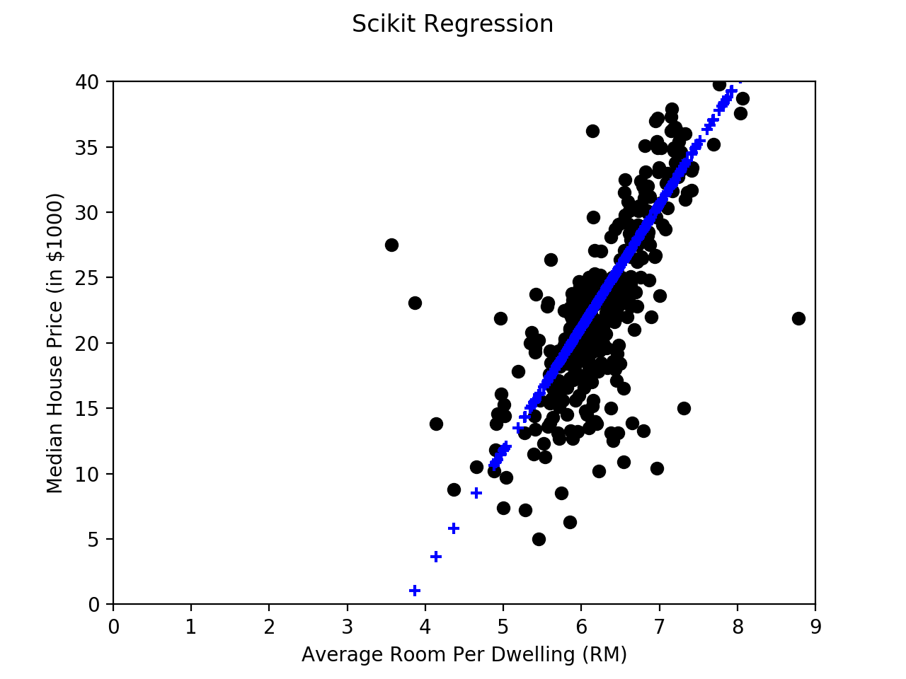
The housing price predictor built in the previous post used Python to run a linear regression over sample data using the scikit-learn package. Once the linear regression process discovered the best line to represent the relationship between the room count and the median neighborhood house price, we re-created the line in Redis and used Redis to predict unknown housing prices from observed features.
In this post we are going to demonstrate how different toolkits can be used in conjunction with Redis, by reimplementing our linear regression program in R. The following R code will replicate the linear regression performed by our Python code in the previous post:
# load our data
library(MASS)
boston.data <- MASS::Boston

# split the dataframe into train and test data sets
boston.train <- boston.data[1:400, ]
boston.test <- boston.data[401:506, ]

# fit a linear regression using the rm column to our data
boston.lm = lm(medv ~ rm, data=boston.train)

# display model parameters
summary(boston.lm)
Even if you have never worked with R before, the code should be easy to follow. The first part of the program loads our data. The Boston Housing Dataset is a classic data set used in machine learning instruction. R, like many statistical toolkits, include several classic data sets. In the case of R, the Boston Housing Dataset is included in the MASS package, so we must load theMASS package before we can access the data.
The second section of our code splits the housing data into a training set and a test set. Following the methodology used in the Python version, we create a training set from the first 400 data points and reserve the remaining 106 data points for the test set. Since R stores our data as a data frame and not in an array (as scikit does), we can skip the slicing and column extraction we performed in Python that made our room data column more accessible.
The linear regression is performed in R using the built-in linear regression function (lm).
The first parameter to lm is used to describe the predictor and predicted values in the data frame. For this problem, we usemedv ~ rm as we are predicting the median housing price data from the average rooms data.
In the final step of the script, the summary method is used to display the coefficients of the fit line to the user.
Plotting our results and comparing them with the results from the previous code:
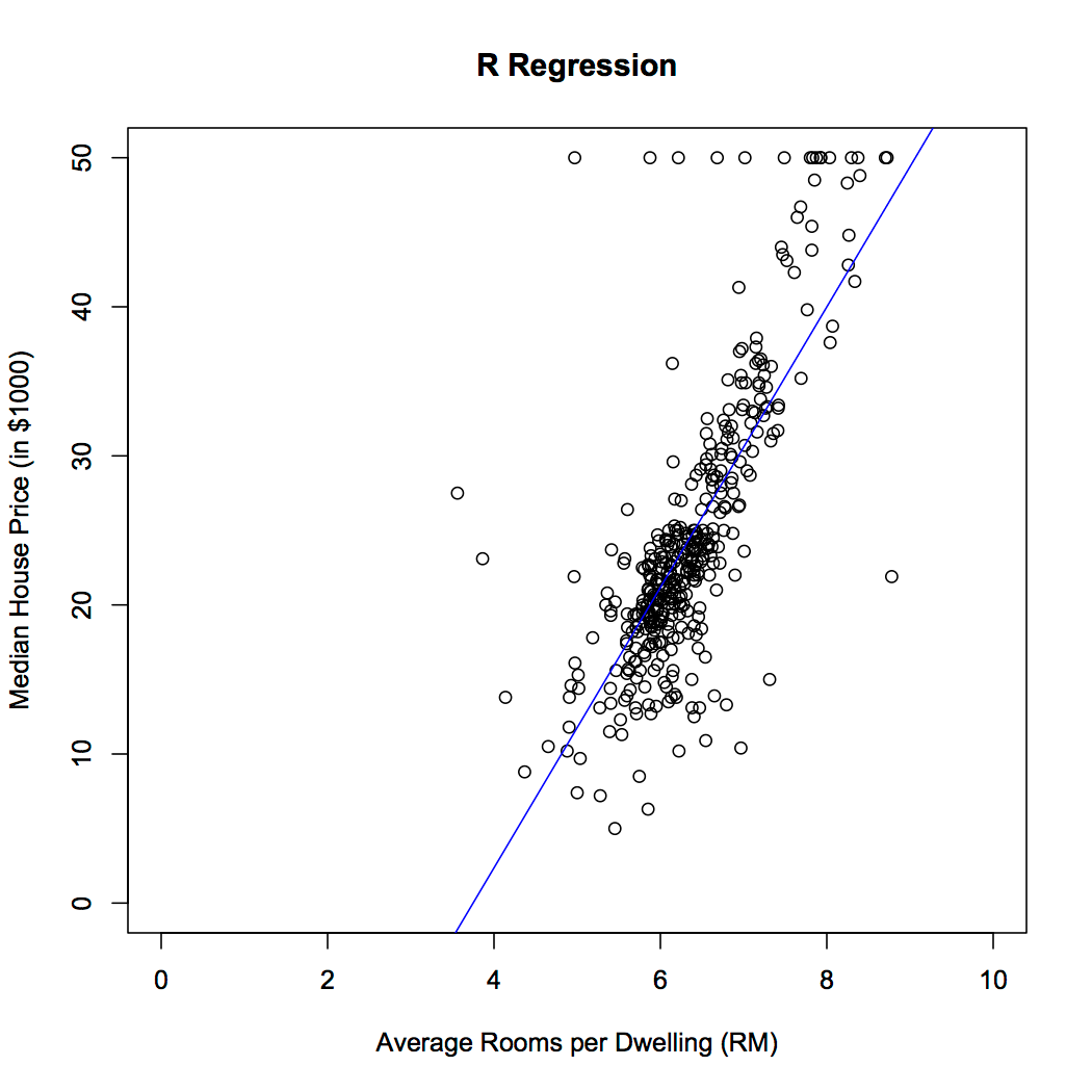
The summary method shows the coefficients determined by the linear regression procedure as:
Coefficients:
            Estimate Std. Error t value Pr(>|t|)
(Intercept) -35.2609     2.6289  -13.41   <2e-16 ***
rm            9.4055     0.4121   22.82   <2e-16 ***
Like the scikit-learn package, R determined the slope of our line to be 9.4055 and the intercept to be -35.2609. Our R code provides identical results to scikit up to the fourth decimal place.
From this point on, the procedure for setting up Redis to predict housing prices is the same as before. First, create a linear regression key using the ML.LINREG.SET command:
127.0.0.1:6379> ML.LINREG.SET boston_house_price:rm-only -35.2609 9.4055
OK
And once the key is created, use the ML.LINREG.PREDICT command to predict housing values:
127.0.0.1:6379>  ML.LINREG.PREDICT boston_house_price:rm-only 6.2
"23.053200000000004”
Once we round the results to four decimal places, we still get an estimated median house price of $23,053 (remember our housing prices are in thousands) for this particular neighborhood.
This may be the first and only time you run R, but the important thing to take away is that the model–not the toolkit–is what is important when using Redis to serve your models.
The other important topic in linear regression that we didn’t cover in our last post is multiple linear regression.
Multiple Linear Regression
In all the examples we have shown so far, we’ve used a single variable to predict a value. Our housing predictor used only the average room size to predict the median housing value, but the data sets have multiple data values (referred to as “features”) associated with a particular median home price.
Linear regression is often performed with multiple variables being used to predict a single value. This gives us a model that looks like y=0+1×1+ … + nxn. In a multiple linear regression we need to solve for an intercept and coefficients for each variable.
The following code implements multiple linear regression, trying to fit a prediction line using all of the available data columns from our Boston Housing Data:
import redis

from sklearn.datasets import load_boston
from sklearn.model_selection import train_test_split
from sklearn.linear_model import LinearRegression

# load out data
boston = load_boston()

# slice the data into train and test sets
x_train = boston.data[:400]
x_test =  boston.data[400:]
y_train = boston.target[:400,]
y_test = boston.target[400:,]

# fit the regression line
lm = LinearRegression()
lm.fit(x_train, y_train)

y_predict = lm.predict(x_test)

coef = lm.coef_
inter = lm.intercept_

for col, c in zip(boston.feature_names, coef):
    print('{colname:7}:\t{coef:0.6f}'.format(colname=col,coef=c))
print("Intercept: {inter}".format(inter=inter))


# set the linear regression in Redis
cmd = ["ML.LINREG.SET", "boston_house_price:full"]
cmd.append(str(inter))
cmd.extend([str(c) for c in coef])

r = redis.StrictRedis('localhost', 6379)
r.execute_command(*cmd)
The table below shows the coefficient scikit determined for the best predictor line. Each coefficient corresponds to a particular variable (feature). For instance, in our multiple linear regression, the constant for average rooms is now 4.887730, instead of the 9.4055 that resulted when only considering the room data.
CRIM   : -0.191246
ZN     : 0.044229
INDUS  : 0.055221
CHAS   : 1.716314
NOX    : -14.995722
RM     : 4.887730
AGE    : 0.002609
DIS    : -1.294808
RAD    : 0.484787
TAX    : -0.015401
PTRATIO: -0.808795
B      : -0.001292
LSTAT  : -0.517954

Intercept: 28.672599590856002
From there, we create a Redis key boston_house_price:full to store our represented multiple linear regression. Keep in mind that Redis doesn’t use named parameters for the arguments to the ML.LINREG commands. The order of the coefficients in the ML.LINREG.SET must match the order of the variable values in the ML.LINREG.PREDICT call. As an example, using the linear regression code above, we would need to use the following order of parameters to our ML.LINREG.PREDICT call:
127.0.0.1:6379> ML.LINREG.PREDICT boston_house_price:all <CRIM> <ZN> <INDUS> <CHAS> <NOX> <RM> <AGE> <DIS> <RAD> <TAX> <PTRATIO> <B> <LSTAT>
This post demonstrated toolkit independence and explained multiple linear regression, to round out our first post on linear regression. We revisited our housing price predictor and “rebuilt” it using R instead of Python to implement the linear regression phase.
R applied the same mathematical models to the housing problem as scikit and learned the same parameters for the line. From there, it was a nearly identical procedure to set up the key in Redis and deploy Redis as a prediction system.
In the next post, we’ll look at logistic regression and how Redis can be used to build a robust classification engine. We promise. In the meantime, connect with the author on twitter (@tague) if you have questions regarding this or previous posts.