
Today we are happy to announce the general availability (GA) of RedisTimeSeries v1.0. RedisTimeSeries is a Redis module developed by Redis Labs to enhance your experience managing time series data with Redis. We released RedisTimeSeries in preview/beta mode over six months ago, and appreciate all the great feedback and suggestions we received from the community and our customers as we worked together on this first GA version. To mark this release, we performed a benchmark, which achieved 125K queries per second with RedisTimeSeries as compared to other time series approaches in Redis. Skip ahead for the full results, or take a moment to first learn about what led us to build this new module.
Why RedisTimeSeries?
Many Redis users have been using Redis for time series data for almost a decade and have been happy and successful doing so. As we will explain later, these developers are using the generic native data structures of Redis. So let’s first take a step back to explain why we decided to build a module with a dedicated time series data structure.
In the DB-engines trend chart below, you can see that time series databases have gained the most in popularity recently. In addition to the ever-growing amounts of data and new time series use cases for self-driving cars, algorithmic trading, smart homes, online retail and more, we believe there are two main technological reasons for this trend.
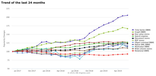
The first reason is that the query pattern and scale of time series data differs from what existing database technologies were built for. While most databases were designed to serve more reads than writes, time series use cases have a high ingestion rate of large volumes of data, and a lower number of read queries. In a root cause analysis use case, reads are sporadic and only touch upon random parts of the data set. In the use case of training AI models (e.g., for anomaly detection in sensor data), typically reads would span a larger part of the data set but still occur significantly less frequently than writes. Because of Redis’ scalable architecture, which delivers high write throughput with low latency, Redis is natural fit for current time series query patterns.
The second reason for this trend is that the toolset required for working with time series is not present in traditional database technologies. Efficient use of resources requires several structural changes, such as automatic downsampling of historical time series data and double delta encoding, as well as features for intuitively querying and aggregating time series data. Traditional database technologies introduce a lot of effort on the application side to address features like retention, downsampling and aggregations.
At RedisLabs, we are strong believers in eating our own dog food. For our cloud offering (which manages over 1 million Redis databases running on thousands of Redis Enterprise clusters), we collect metrics from each cluster inside an internal Redis database. During an internal project to enhance our own infrastructure metrics, we experienced first-hand the limitations and development effort of using core Redis data structures for time series use cases. We figured there must be a better and more efficient way. In addition to the toolset-specific features above, we also wanted out-of-the-box secondary indexing so we could query time series sets efficiently.
Time series with core Redis data structures
There are two ways to use time series in Redis while reusing existing data structures: Sorted Sets and Streams. Many articles explain how to model time series with Redis core data structures. Below are some of the key principles we’ll use later in our benchmark.
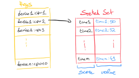
Sorted Sets
A Sorted Set stores values by their scores. In the case of time series data, the score is the timestamp on which an event was observed. The value repeats the timestamp followed by a separator and the actual measurement, e.g. “<timestamp>:<measurement>”. This is done because each value in a sorted set should be unique. Alternatively, the value holds the name of a unique key, which stores a hash where more data or measurements can be kept for the given timestamp.
Downsides of this approach:
- Sorted Sets are not a memory-efficient data structure
- Insertion is O(log(N)), so it takes longer to insert, the larger the set becomes
- It’s missing a time series toolset
Streams

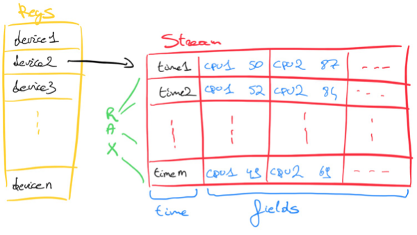
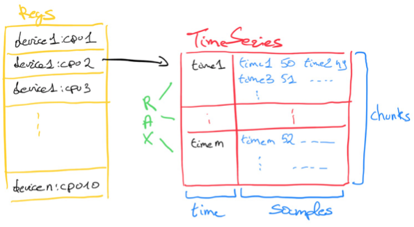
Redis Streams, the most recently added data structure (and hence currently less frequently used for time series), consumes less memory than Sorted Sets and is implemented using Rax (a separate implementation of Radix trees). In general, Redis Streams enhances the performance of insertion and reads compared to Sorted Sets, but still misses a toolset specific to time series, since it was designed as a generic data structure.
Downsides of this approach:
- It’s missing a time series toolset
RedisTimeSeries capabilities
In RedisTimeSeries, we are introducing a new data type that uses chunks of memory of fixed size for time series samples, indexed by the same Radix Tree implementation as Redis Streams. With Streams, you can create a capped stream, effectively limiting the number of messages by count. In RedisTimeSeries, you can apply a retention policy in milliseconds. This is better for time series use cases, because they are typically interested in the data during a given time window, rather than a fixed number of samples.
Downsampling / compaction
If you want to keep all of your raw data points indefinitely, your data set will grow linearly over time. However, if your use case allows you to have less fine-grained data further back in time, downsampling can be applied. This allows you to keep fewer historical data points by aggregating raw data for a given time window using a given aggregation function. RedisTimeSeries supports downsampling with the following aggregations: avg, sum, min, max, range, count, first and last.
Secondary indexing
When using Redis’ core data structures, you can only retrieve a time series by knowing the exact key holding the time series. Unfortunately, for many time series use cases (such as root cause analysis or monitoring), your application won’t know the exact key it’s looking for. These use cases typically want to query a set of time series that relate to each other in a couple of dimensions to extract the insight you need. You could create your own secondary index with core Redis data structures to help with this, but it would come with a high development cost and require you to manage edge cases to make sure the index is correct.
RedisTimeSeries does this indexing for you based on `field value` pairs (a.k.a labels) you can add to each time series, and use to filter at query time (a full list of these filters is available in our documentation). Here’s an example of creating a time series with two labels (sensor_id and area_id are the fields with values 2 and 32 respectively) and a retention window of 60,000 milliseconds:
TS.CREATE temperature RETENTION 60000 LABELS sensor_id 2 area_id 32
Aggregation at read time
When you need to query a time series, it’s cumbersome to stream all raw data points if you’re only interested in, say, an average over a given time interval. RedisTimeSeries follows the Redis philosophy to only transfer the minimum required data to ensure lowest latency. Below is an example of aggregation query over time buckets of 5,000 milliseconds with an aggregation function:
127.0.0.1:6379> TS.RANGE temperature:3:32 1548149180000 1548149210000 AGGREGATION avg 5000

1) 1) (integer) 1548149180000

2) "26.199999999999999"

2) 1) (integer) 1548149185000

2) "27.399999999999999"

3) 1) (integer) 1548149190000

2) "24.800000000000001"

4) 1) (integer) 1548149195000

2) "23.199999999999999"

5) 1) (integer) 1548149200000

2) "25.199999999999999"

6) 1) (integer) 1548149205000

2) "28"

7) 1) (integer) 1548149210000

2) "20"
Integrations
RedisTimeSeries comes with several integrations into existing time series tools. One such integration is our RedisTimeSeries adapter for Prometheus, which keeps all your monitoring metrics inside RedisTimeSeries while leveraging the entire Prometheus ecosystem.
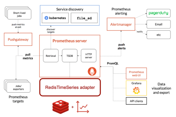
Furthermore, we also created direct integrations for Grafana and Telegraph. This repository contains a docker-compose setup of RedisTimeSeries, its remote write adaptor, Prometheus and Grafana. It also comes with a set of data generators and pre-built Grafana dashboards.
Benchmark
To demonstrate the full power of our newly GA RedisTimeSeries module, we benchmarked it against three common techniques for handling time series data. We used a client-server setup with two separate machines in order to compare the performance of Sorted Sets, Streams and RedisTimeSeries for ingestion, query time and memory consumption.
Specifically, our setup included:
- Client and server: AWS c5.18xl
- Redis Enterprise version 5.4.4-7
- A Redis Enterprise database with 16 shards and 48 proxy threads
- A data set with:
- 4,000 devices, 10 metrics per device
- Each metric is a CPU measurement
- 10,800 samples per metric (every 10 seconds for 30 hours)
- 43,200,000 samples in total
Data modelling approaches
Redis Streams allows you to add several field value pairs in a message for a given timestamp. For each device, we collected 10 metrics that were modelled as 10 separate fields in a single stream message.
For Sorted Sets, we modeled the data in two different ways. For “Sorted Set per Device”, we concatenated the metrics and separated them out by colons, e.g. “<timestamp>:<metric1>:<metric2>: … :<metric10>”.
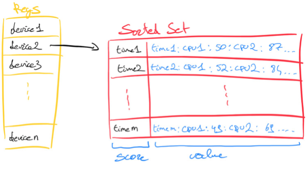
Of course, this consumes less memory but needs more CPU cycles to get the correct metric at read time. It also implies that changing the number of metrics per device isn’t straightforward, which is why we also benchmarked a second Sorted Set approach. In “Sorted Set per Metric,” we kept each metric in its own Sorted Set and had 10 sorted sets per device. We logged values in the format “<timestamp>:<metric>”.
Another alternative approach would be to normalize the data by creating a hash with a unique key to track all measurements for a given device for a given timestamp. This key would then be the value in the sorted set. However, having to access many hashes to read a time series would come at a huge cost during read time, so we abandoned this path.
In RedisTimeSeries, each time series holds a single metric. We chose this design to maintain the Redis principle that a larger number of small keys is better than a fewer number of large keys.
It is important to note that our benchmark did not utilize RedisTimeSeries’ out-of-the-box secondary indexing capabilities. The module keeps a partial secondary index in each shard, and since the index inherits the same hash-slot of the key it indices, it is always hosted on the same shard. This approach would make the setup for native data structures even more complex to model, so for the sake of simplicity, we decided not to include it in our benchmarks. Additionally, while Redis Enterprise can use the proxy to fan out requests for commands like TS.MGET and TS.MRANGE to all the shards and aggregate the results, we chose not to exploit this advantage in the benchmark either.
Data ingestion
For the data ingestion part of our benchmark, we compared the four approaches by measuring how many devices’ data we could ingest per second. Our client side had 8 worker threads with 50 connections each, and a pipeline of 50 commands per request.
| Redis Streams | RedisTimeSeries | Sorted Set per Device |
Sorted Set per Metric |
|
| Command | XADD | TS.MADD | ZADD | ZADD |
| Pipeline | 50 | 50 | 50 | 50 |
| Metrics per request | 5000 | 5000 | 5000 | 500 |
| # keys | 4000 | 40000 | 4000 | 40000 |
Table 1: Ingestion details of each approach
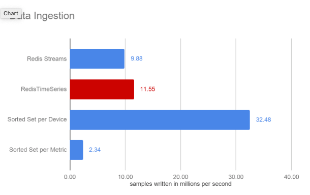
All our ingestion operations were executed at sub-millisecond latency and, although both used the same Rax data structure, the RedisTimeSeries approach has slightly higher throughput than Redis Streams.
As can be seen, the two approaches of using Sorted Sets yield very different throughput. This shows the value of always prototyping an approach against a specific use case. As we will see on query performance, the Sorted Set per Device comes with improved write throughput but at the expense of query performance. It’s a trade off between ingestion, query performance and flexibility (remember the data modeling remark we made earlier) for your use case.
Read performance
The read query we used in this benchmark queried a single time series and aggregated it in one-hour time buckets by keeping the maximum observed CPU percentage in each bucket. The time range we considered in the query was exactly one hour, so a single maximum value was returned. For RedisTimeSeries, this is out of the box functionality (as discussed earlier).
TS.RANGE cpu_usage_user{1340993056} 1451606390000 1451609990000 AGGREGATION max 3600000
For the Redis Streams and Sorted Sets approaches, we created the following LUA scripts. The client once again had 8 threads and 50 connections each. Since we executed the same query, only a single shard was hit, and in all four cases this shard maxed out at 100% CPU.
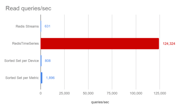
This is where you can see the real power of having dedicated data structure for a given use case with a toolbox that runs alongside it. RedisTimeSeries just blows all other approaches out of the water, and is the only one to achieve sub-millisecond response times.
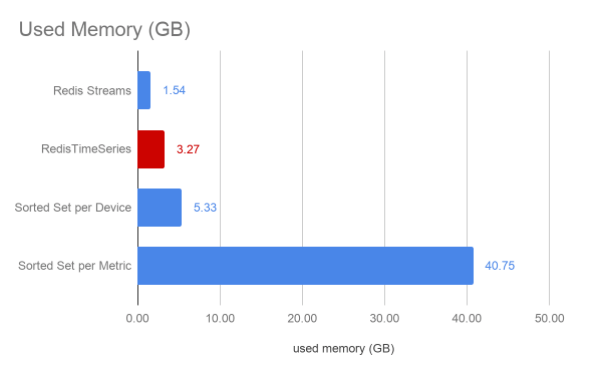
Memory Utilization
In both the Redis Streams and Sorted Set approaches, the samples were kept as a string, while in RedisTimeSeries it was a double. In this specific data set, we chose a CPU measurement with rounded integer values between 0-100, which thus consumes two bytes of memory as a string. In RedisTimeSeries, however, each metric had 64-bit precision.
RedisTimeSeries can be seen to dramatically reduce the memory consumption when compared against both Sorted Set approaches. Given the unbounded nature of time series data, this is typically a critical criteria to evaluate – the overall data set size that needs to be retained in memory. Redis Streams reduces the memory consumption further but would be equal or higher than RedisTimeSeries when more digits for a higher precision would be required.
Conclusion
When choosing your approach, you need to understand the ingestion rate, query workload, overall data set size and memory footprint of your time series use case. There are several approaches for modeling time series data in Redis as we have seen, each with different characteristics. RedisTimeSeries provides a new approach that treats time as a first class citizen and comes with an out-of-the-box time series toolkit as described earlier. It combines efficient memory usage with extraordinary query performance, with a small overhead during ingestion. This turns the desire for real-time analytics of time series data into a reality.
Next steps
We are happy with what we achieved in our 1.0 GA version of RedisTimeSeries, but this is only the beginning. We would love to hear your feedback, so we can incorporate it into our roadmap. In the meantime, here’s the list of things we’re planning next:
- Double delta encoding of timestamps / measurements. This will significantly reduce the amount of memory consumed per observed measurement, making RedisTimeSeries a better option than Redis Streams if memory utilization is important.
- More integrations for existing visualization libraries, sinks from stream providers, and also native integration for RDBTools.
- Convenient migration tooling from other databases.
- Support for Redis on Flash, so we can keep historical data on slower storage.
We strongly believe that all Redis users with time series use cases will benefit from using RedisTimeSeries. If you’re still not convinced and want to try it out yourself, here’s a quickstart guide.
Sponsored by Redis Labs