MOTIVATION: SUPPORTING HIGH DATA INGESTION RATES AND PERFORMING FREQUENT AGGREGATE QUERIES

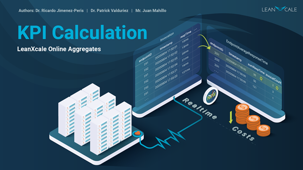
In real time analytics, a major requirement is to be able to ingest data at high rates, while at the same time compute aggregations over the real-time data. For instance, a common use case is ingesting data at high rates and computing KPIs or other metrics, over the ingested data. Examples of this use case are performance monitoring, IoT, eAdvertisement, smart grids, industry 4.0, etc. This kind of workload is troublesome for SQL databases because they are not efficient at ingesting data. Also, the aggregate analytical queries are very expensive because they need to traverse large amounts of data very frequently. NoSQL databases (see our blog post on NoSQL), in particular key-value data stores, are good at ingesting data more efficiently and handle that part of the workload. However, they are not good at analytical queries, if at all supported. As a result, it is very common to find solutions that need:

• To pre-compute aggregations at the application level to persist them later. This approach is arduous to develop and has limitations in both the durability guarantees (a crash will cause the loss of all aggregations) and its scalability (when the amount of data to aggregate requires more than one server).
• Or to combine different data management technologies to solve this use case. This yields complex architectures that require a lot of talent to be created successfully and are not only very hard to develop, but also very hard to maintain.

WHY ONLINE AGGREGATES

One differential key feature of LeanXcale is online aggregates. LeanXcale has developed a new technology based on a brand new semantic multi-version concurrency control (patent pending) that enables it to compute aggregates in an incremental and real-time manner, using aggregate tables. As data are ingested, it becomes possible to update the relevant aggregate tables, so aggregates are always pre-computed. Thus, the formerly complex developments or architectures become a basic architecture with almost costless queries, that read one or more rows of an aggregate table. Data ingestion becomes slightly more expensive but removes the cost of computing the aggregates. In the following example, we motivate the concept of online aggregates by showing that a NoSQL data store or a traditional SQL database cannot solve the problem. Then we explain how the new technology from LeanXcale succeeds at solving this use case.

USE CASE EXAMPLE: APPLICATION PERFORMANCE MONITORING (APM)

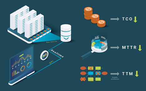
In application performance monitoring, it is very important to detect anomalies in the application behavior as soon as they happen, in order to reduce the Mean-Time-To-Repair (MTTR). Typically, the behavior is modelled by at least two metrics: number of invocations and average response time.

Since these events are asynchronous, they are aggregated frequently with a temporal criterium to simplify their management in dashboarding or to define the threshold of what is considered an anomaly. Commonly, it is also necessary to know these metrics at different aggregation levels: customer, application, application server, and endpoint (e.g., a REST API endpoint or any other user actionable unit).

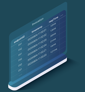
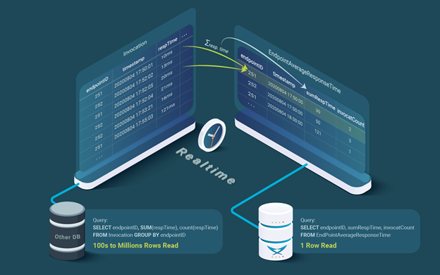
In this example, we describe how to compute this aggregation hierarchy in real-time in a totally accurate and inexpensive way. We maintain an invocation table for tracking the endpoint invocations in real-time (see Table 1). Each invocation row contains the timestamp of the invocation, the response time, the endpoint, and any other information of interest that we do not detail here.

We need a reference to determine if the endpoint 251 invocation at 17:55:03 is working correctly. We use a simple model, taking as a threshold an anomalous response time two times the average response time of the previous period. In this case, in the period [17:50-17:55[ the response times recorded were 10 and 20, yielding an average of 15 ms. The response time at 17:55:03 is 121ms > 2x15ms=30 ms, so it is considered anomalous. More complex models take into consideration application, infrastructure, or temporal criteria.

In a SaaS platform, this would mean aggregating several million rows per second.  Let’s think that this tool should be ready to aggregate invocations and calculate average response time for any generic endpoint.

USING AGGREGATE TABLES

One way to reduce the cost of the aggregation calculation would be to compute aggregates incrementally in aggregate tables. We could have an aggregate table per aggregation level. In our example, we have the invocation table and the threshold aggregation table. Although, as commented, in the real use case, more aggregation levels will be needed for different time periods and different aggregation levels according to the customer application hierarchy. This aggregation table (see

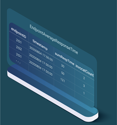
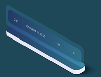
Then, every time an endpoint is invoked, an invocation row is added to the invocation table as part of the same transaction and the corresponding row of the EndpointAverageResponseTime aggregate table is updated. In the aggregation EndpointAverageResponseTime table, we would update the row with the associated endpoint and timestamp, updating the value by adding the new response time to the sumRespTime column and incrementing the number of invocations column by one. Table 1 depicts an example of a few rows of the table. After getting the metric: (251, 20200804 17:50:01, 10), and before getting the metric (251, 20200804 17:52:05, 20), the row for (251, 20200804, 17:50:00) in the EndpointAverageResponseTime aggregation table would be the one depicted in Figure 1.

Table 2) would have the endpointID (an integer) as key and the timestamp (day, month, year, hour, minute, second) of the start of each 5-minute interval. Then, every time an endpoint is invoked, an invocation row is added to the invocation table as part of the same transaction and the corresponding row of the EndpointAverageResponseTime aggregate table is updated. In the aggregation EndpointAverageResponseTime table, we would update the row with the associated endpoint and timestamp, updating the value by adding the new response time to the sumRespTime column and incrementing the number of invocations column by one. Table 1 depicts an example of a few rows of the table. After getting the metric: (251, 20200804 17:50:01, 10), and before getting the metric (251, 20200804 17:52:05, 20), the row for (251, 20200804, 17:50:00) in the EndpointAverageResponseTime aggregation table would be the one depicted in Figure 1.

After the metric (251, 20200804 17:52:05, 20) is inserted in the Invocation table, we would update the above row in the EndpointAverageResponseTime aggregation table by adding 20 to the sumRespTime column yielding 30 (10+20) and incrementing the invocatCount column by one; yielding 2 (1+1) that would result in the row shown in Figure 2.

PROBLEMS WHEN COMPUTING AGGREGATE TABLES WITH NOSQL DATA STORES

What happens if we implement the aggregate tables with a NoSQL data store? Let’s see. If there are two concurrent invocations over the same endpoint aggregation row (in fact, there will be thousands to millions of concurrent readings over the same endpoint), and both are allowed to proceed, one of them would be lost.

This is called the “Lost Updates” anomaly [Özsu & Valduriez 2020]. To update the aggregation row for endpoint 252 and timestamp 20200804 17:50:00, we would execute a Get using (252, 20200804 17:50:00) as key and then execute a Put with (252, 20200804 17:50:00) as key with the aggregated value incremented with the response time and number of invocations.

Let ‘s consider a concrete example. In the EndpointAverageResponseTime aggregation table, there is an aggregation row every five minutes for endpoint 252, say (252, 20200804 17:52:02, 13, 1). Now, two invocations happen concurrently for endpointID 252 (in fact thousands or millions of concurrent invocations, but we’ll focus on just two concurrent invocations) with response times 21 and 16 within the 5-minute interval [20200804 17:50:00, 20200804 17:55:00]. Now, we insert a new row into the invocation table for each of them: (252, 20200804 17:52:04, 21) and (252, 20200804 17:53:21, 16). For each invocation, we have to update the endpoint aggregation table.

Let’s look at what happens in the EndpointAverageResponseTime aggregation table. Assume the following interleaving happens in the update of the endpoint: (252, 20200804 17:50:00) aggregation row in the EndpointAverageResponseTime aggregation table. The two updates do the Get with (252, 20200804 17:50:00) as key. Both will read the row (252, 20200804 17:50:00, 13, 1). One of them will do a Put(252, 20200804 17:50:00, 34, 2) and the other will do a Put(252, 20200804 17:50:00, 29, 2).

One of them will be processed first and the other, second. Assume the first one processed is Put(252, 20200804 17:50:00, 34, 2). Now the data store will contain that row. Then, the data store processes Put(252, 20200804 17:50:00, 29, 2). What happened? The second Put erased the effect of the first Put. The reason is that the Put are blind writes, they write a value independently of what is already stored.

PROBLEMS IN DOING AGGREGATE TABLES WITH SQL DATABASES

We can avoid the “Lost Updates” problem using an SQL database with ACID transactions. With an SQL database, each endpoint invocation would be a transaction where we insert an invocation row in the invocation table and update the corresponding aggregation row in the endpoint table:

INSERT INTO Invocations (endpointID, timestamp, respTime) 
              VALUES (252, "20200804 17:52:04”, 21);
SELECT sumRespTime, invocatCount FROM EndpointAverageResponseTime WHERE (endpointID = 252 AND timestamp = "20200804 17:50:00");
The select will return after the first update (34, 2), and we write the updated value: (34+16=50, 2+1=3): 
UPDATE EndpointAverageResponseTime SET sumRespTime=50, invocatCount=3 WHERE (endpointID=252 AND timestamp = "20200804 17:50:00");
COMMIT;

SQL databases avoid the “Lost Updates” problem by means of transactional concurrency control. There are two popular kinds of concurrency control: multiversioning and locking. Both will avoid the “Lost Updates” but will introduce a contention problem. We exemplify that now with multiversion concurrency control.

The concurrency control forbids two concurrent transactions (two transactions that overlap in time) to modify the same row. Thus, in the aforementioned example of the two concurrent transactions for endpointID = 252 and timestamp = 20200804 17:50:00, one transaction would be rollbacked. If there are more than two transactions in parallel updating the same aggregation row, then all transactions but one would be rollbacked.

This means that the concurrency control solves the inconsistency problem of the “Lost Updates” but introduces a huge contention problem that makes it useless for the target use case. With locking, all transactions will be waiting for each other, since they would block on updating the row in the aggregation table and would have to execute and commit sequentially, resulting in a high contention.

LEANXCALE SOLUTION: ONLINE AGGREGATES

How does LeanXcale solve the problem? With a new technology based on a patent-pending semantic multiversion concurrency control. In this new concurrency control, writes are not blind. The writes would actually carry the operation to be performed, e.g., Sum(10) and Sum(20) for sumRespTime column in the above example. Since additions are commutative, they do not conflict as far as one keeps track that they are additions until the corresponding version of the row is generated. In order to attain data consistency and, in particular, the expected data consistency in multiversion concurrency control (snapshot isolation), one has to be really smart when handling multiversioning.

This is exactly what the technology developed by LeanXcale does. LeanXcale’s distributed storage layer, KiVi, supports a new kind of column, aggregate columns (also called delta columns), which adopt this new semantic multiversion concurrency control and enable online aggregates. What is interesting is that this feature can be combined with the linear scalability of LeanXcale (see our blog post on Understanding Scalability).

HOW ONLINE AGGREGATES WORK? OPERATION ROWS (DELTAS)

Aggregate columns are conflictless. The way versions are handled is as follows. Two kinds of rows are considered: regular rows or value rows. That is, rows that contain values as in any traditional database, and operation rows (also called deltas) that represent operations to be performed over the columns of the rows, e.g., (252, 20200804 17:50:00, Sum(21), Sum(1), CTS=1). One key problem is that, since operations are conflictless, there might be gaps in the commit order, so in general it is not possible to generate value rows for each operation row at the time a transaction with operation rows is committed.

HOW ONLINE AGGREGATES WORK? GETTING MULTIVERSIONING RIGHT IS NOT EASY

Let’s examine the previous example. Assume, in the above example, that the transaction with the measure of 21ms is t1 and that with the measure of 16ms is t2. Assume that t1 commits first and the transaction that commits second is t2. In multiversion concurrency control, rows are labeled with the commit timestamp (CTS). The commit timestamp is just an integer that is increased monotonically and determines the commit order. Assume that the worst case happens and t1 gets a CTS 2 and t2 gets a CTS 1. If a transaction t3 is started after the commit of t1 and before the commit of t2, it would get a start timestamp (i.e., snapshot) of 0, that is, the snapshot before both t1 and t2, to guarantee that it does not observe any gap in the commit order. If it got the snapshot at timestamp 2, it would miss the updates from the transaction with CTS 1, which would violate snapshot isolation.

HOW ONLINE AGGREGATES WORK? HANDLING MULTIVERSIONING RIGHT

LeanXcale solves the problem by converting operation rows into value rows only when the snapshot of the database is beyond the commit timestamp of the operation rows. This approach guarantees that the serialization order is gap free and therefore the generated versions are guaranteed to be consistent and in accordance with the semantics of snapshot isolation. In the previous example, the EndpointAverageResponseTime aggregation table contains the row (252, 20200804 17:50:00, 13, 1, CTS=0). When the snapshot of the database reaches timestamp 1, then the operation row from t2 adding 21 to sumRespTime and 1 to invocatCount will be converted into the value row (252, 20200804 17:50:00, 34, 2, CTS=1). When the snapshot reaches timestamp 2, then the operation row from t1 adding 16 to sumRespTime and 1 to invocatCount is applied to the latest value row (the one generated by t2), yielding the following value row: (252, 20200804 17:50:00, 50, 2, CTS=2). In this way, all the versions needed by the different snapshots are generated consistently, thus fulfilling the snapshot isolation semantics.

LEANXCALE COMPETITIVENESS

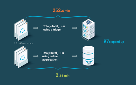
In order to provide a comparison point against state of the art technology, we compared LeanXcale online aggregates against doing aggregates with PostgreSQL. The way to do aggregates with a traditional SQL database is to perform them via triggers. In the comparison, aggregates are implemented with PostgreSQL using triggers. In the case of LeanXcale the aforementioned online aggregates are used. As can be seen in Figure 4, LeanXcale outperformed PostgreSQL by almost two orders of magnitude, 97 times.

MAIN TAKEAWAYS

Monitoring tools need to ingest data at high rates and compute aggregations at the same time. These tools commonly use a combination of in memory data structures with persisted information to provide dashboards, forecasts, or identify anomalies. NoSQL or SQL are not efficient with these aggregation tables.  They get very complex and hard to maintain and have issues with durability of the data, seeing as, when there is a failure, the part stored only in the memory part is lost and cannot be recovered. Using a solution that guarantees durability in the event of failures with a NoSQL data store does not work since the aggregations get the “Lost Updates” inconsistency problem. Whereas with an SQL database, one gets high contention. Thus, tailor-made applications or complex architectures combining different database technologies have to manage the computation of aggregates. Ultimately, incrementing the development and maintaining costs.

LeanXcale has solved the problem with a (patent pending) technology, online aggregates, based on a new semantic multiversion concurrency control. With this new semantic multiversion control, there are neither “Lost Updates” inconsistencies (as in NoSQL) nor contention (as in SQL). However, at the same time, full ACID consistency as mandated by Snapshot Isolation is provided.

LeanXcale solves this common use case in a highly efficient manner. Consequently, the formerly expensive architectures or applications become quite simple due the fact that the database manages all the complexity. This technology provides a multiplier effect in conjunction with the linear horizontal scalability: Developers only have to create aggregation tables, ingest and perform regular gets, and they can use it at any scale.

REFERENCES

[Özsu & Valduriez 2020] Tamer Özsu, Patrick Valduriez. Principles of Distributed Database Systems, 4th Edition, Springer, 2020.

RELATED BLOG POSTS

ABOUT THIS BLOG SERIES

This blog series aims at educating database practitioners on the differential features of LeanXcale, taking a deep dive on the technical and scientific underpinnings. The blog provides the foundations on which the new features are based and provides the reader with facts, allowing them to compare LeanXcale to existing technologies and learn its real capabilities.

ABOUT THE AUTHORS

• Dr. Ricardo Jimenez-Peris is the CEO and founder of LeanXcale. Before founding LeanXcale, for over 25 years he was a researcher in distributed database systems, director of the Distributed Systems Lab and a university professor teaching distributed systems.
• Dr. Patrick Valduriez is a researcher at Inria, co-author of the book “Principles of Distributed Database Systems” that has educated legions of students and engineers in this field and, more recently, Scientific Advisor of LeanXcale.
• Mr. Juan Mahillo is the CRO of LeanXcale and a former serial Entrepreneur. After selling and integrating several monitoring tools for the biggest Spanish banks and telco with HP and CA, he co-founded two APM companies: Lucierna and Vikinguard. The former was acquired by SmartBear in 2013 and named by Gartner as Cool Vendor.

ABOUT LEANXCALE

LeanXcale is a startup making an ultra-scalable NewSQL database that is able to ingest data at the speed and efficiency of NoSQL and query data with the ease and efficiency of SQL. Readers interested in LeanXcale can visit the LeanXcale website.

Sponsored by LeanXcale