SCALABLE GIS ON LEANXCALE

WRITTEN BY LEANXCALE TEAM

New applications, such as geo-marketing tools, car-sharing, or mobility apps, require handling large data volumes. Traditionally, most applications that require geographical query capabilities use PostgreSQL as a database. However, because PostgreSQL is a centralized database, its scalability capacities are limited. This post introduces LeanXcale as a scalable alternative for developers that process geographical data.

INTRODUCTION

LeanXcale’s GIS support combined with LeanXcale’s performance capacity result in a high-performance GIS system that allows a large volume of data and a high number of parallel queries to be harnessed effectively. Now, LeanXcale’s GIS support means it can process geographical operations as well as offer high-performance query behavior. This has been done thanks to three different aspects:

• A radical data-store design made to provide optimal efficience.
• A fully distributed database architecture that allows scaling-out.
• A new geohash-based filtering algorithm specially designed to act over queries with geographical where clauses. 

THE SECRET SAUCE

A few weeks ago, we explained in this article how to use GIS support in LeanXcale to draw vehicle positions on a map, to illustrate its capacity of handling and processing geographical data. But being able to support geographical data and operations is not enough; it is necessary to do it offering high performance for any data or parallel queries volume. Now, we would like to go one step further and have a look at LeanXcale’s performance when harnessing bigger datasets containing geographical information. In this journey, we will compare Postgres and LeanXcale with different dataset sizes. LeanXcale’s outstanding performance is based on three different aspects:

GEO-HASH

One of the aspects that cause this LeanXcale performance improvement over GIS data has been made by the design and implementation of a new filtering algorithm based on what is called Geohash. Geohash is a public domain geocode system invented in 2008 by Gustavo Niemeyer and (similar work in 1966) G.M. Morton, which encodes a geographic location into a short string of letters and digits. Geohashes offer properties like arbitrary precision and the possibility of gradually removing characters from the end of the code to reduce its size (and gradually lose precision). LeanXcale can use this gradual precision degradation to perform certain ST operations over geographical data, following the Geohash principle that specifies that nearby places will often present similar prefixes. 

KIVI

KiVi is a low-latency relational key-value data-store. It offers a disruptive design mono-thread per core design that avoids thread context switches, thread synchronization, and NUMA remote memory access, making it extremely efficient and cost-effective. KiVi takes advantage of the IO of the fastest storage device, but it doesn’t have a special requirement. KiVi is the perfect data store to provide the scan performance that a GIS database requires.

DISTRIBUTED ARCHITECTURE

LeanXcale is a relational SQL engine, with a similar interface than PostgreSQL. LeanXcale is a fully distributed database. All its layers: its data storage, its transactional engine, and its SQL engine can be deployed from one to n instances, providing a linear scalability maintaining all the ACID capacities. LeanXcale behavior scales for big data and for number of parallel queries.

Focusing on the dataset size:The most popular GIS capabilities database, PostgreSQL, scale out based on having a unique write node and several read replicas. In other words, a table is fully replicated in all the nodes. The bigger a table is, the longer a scan query lasts. A 100 million rows table is a challenge for this structure.

On the other hand, LeanXcale splits the table in several pieces in the different data-stores (KVDS). This capacity allows parallel scanning and with the right data partitioning and optimal performance, no matter the size of the dataset. Additionally, LeanXcale can provide active-active HA.

THE BENCHMARK

COMPONENTS

To perform our benchmark test, we need:

• A dataset containing geographical-based information, with a significant amount of data.
• A LeanXcale (LX) database instance. You can find it here.
• Another database with GIS support. The most popular database with GIS support today is PostgreSQL, which includes the PostGIS extension to handle geometry and geography types, as well as a complete set of ST functions to perform geographical operations.

Referring to the dataset, we again resorted to this research group’s work and found a reference to Brian Donovan and Daniel B. Work paper “New York City Taxi Trip Data (2010-2013)” from the University of Illinois. The dataset was obtained through a Freedom of Information Law (FOIL) request from the New York City Taxi & Limousine Commission (NYCT&L). Thanks to a generous hosting policy by the University of Illinois at Urbana-Champaign, this large dataset is publicly available, and you can find it here.

The dataset is organized as CSV files with the following column structure:

• medallion: a permit to operate a yellow taxicab in New York City, which is effectively a (randomly assigned) car ID.
• hack license: a license to drive the vehicle, which is effectively a (randomly assigned) driver ID.
• vendor_id: e.g., the Verifone Transportation Systems (VTS), or Mobile Knowledge Systems Inc (CMT).
• rate_code: the taximeter rate, see NYCT&L description.
• store_and_fwd_flag: an unknown attribute.
• pickup_datetime: start time of the trip, mm-dd-yyyy hh24:mm:ss EDT.
• dropoff_datetime: end time of the trip, mm-dd-yyyy hh24:mm:ss EDT.
• passenger_count: the number of passengers on the trip, the default value is one.
• trip_time_in_secs: the trip time measured by the taximeter in seconds.
• trip_distance: the trip distance measured by the taximeter in miles.
• pickup_longitude and pickup_latitude: the GPS coordinates at the start of the trip.
• dropoff_longitude and dropoff_latitude: the GPS coordinates at the end of the trip.

The interesting fields for this article are pickup_longitude and pickup_latitude. We selected the data corresponding to 2013 to perform this benchmark (~165 million rows).

Regarding the LeanXcale database instance, we deploy an instance with one meta node and eight data nodes. As described in our other articles, a single data node is composed of a Query Engine, a Logger Process, and, the most important for our current purpose, a Kivi Data Store. Kivi, the LeanXcale storage engine, can be fully distributed as all the tables are split and distributed across many instances. Consequently, the storage engine can run on many nodes without any tradeoffs. 

So, we have:

• One AWS machine, type “m5.xlarge,” with four virtual CPUs, 16GB RAM, and a 300 GB disk. This machine will host the LeanXcale meta node and four data nodes.
• A second AWS machine with the same capacity as the first, which will store four additional data nodes.

Regarding the PostgreSQL instance, we selected:

• An AWS RDS service with a PostgreSQL 11 instance hosted on a machine with the same power as the LeanXcale instances (4 virtual CPUs, 16GB RAM, and 300 GB disk). 
• Because we use the RDS service, and it is not possible to handle a PostgreSQL cluster, we created a read replica with the same characteristics as the primary instance.

DATABASE STRUCTURE

For both databases, we created a single table, called TRIP_DATA, to store the complete dataset. Taking advantage of everything a database can offer is important to increase performance. As shown in the dataset description, we do not have geographical representations of pickup or dropoff points, but instead, have latitude and longitude data.

For PostgreSQL, we created a new geometry column and trigger to deals with the latitude and longitude conversion to a point type. So, in PostgreSQL, we have the structure:

CREATE TABLE trip_data (
    medallion int4 NOT NULL,
    hack_license int4 NOT NULL,
    vendor_id varchar(3) NOT NULL,
    rate_code int4 NOT NULL,
    store_and_fwd_flag varchar(1),
    pickup_datetime timestamp NOT NULL,
    dropoff_datetime timestamp NOT NULL,
    passenger_count int4 NOT NULL,
    trip_time_in_secs int4 NOT NULL,
    trip_distance float8 NOT NULL,
    pickup_longitude float8 NOT NULL,
    pickup_latitude float8 NOT NULL,
    dropoff_longitude float8,
    dropoff_latitude float8,
    geom_pickup geometry NOT NULL,
    CONSTRAINT trip_data_pkey PRIMARY KEY (geom_pickup,pickup_datetime,medallion,hack_license)

“geom_pickup” is the new column with the representation of pickup_latitude and pickup_longitude as a geometry type point. To enable faster searches, this column is also added as part of the PK. We also define an index over geom_pickup:

CREATE INDEX idx_trip_data_geom_pickup ON trip_data (geom_pickup);

The function used by the trigger to calculate the point is:

CREATE OR REPLACE FUNCTION before_insert_geom_pickup()
    RETURNS trigger
    LANGUAGE plpgsql
AS $function$
BEGIN
    if NEW.geom_pickup is null then
        NEW.geom_pickup = ST_SetSRID(ST_MakePoint(NEW.PICKUP_LONGITUDE,NEW.PICKUP_LATITUDE), 4326);
    end if;
    RETURN NEW;
END;
$function$

For LeanXcale, as we created an additional column for the geometry type in PostgreSQL, we create a new column in LeanXcale to store the geohash representation of the point geometry. This is declared as a constraint that uses LeanXcale’s special “geohash” function. Unlike PostgreSQL, when inserting through SQL in LeanXcale, there is no need to define a trigger as the Query Engine automatically calculates the geohash value of the point resulting from the latitude and longitude columns, and applies the geohash function from the constraint and inserts it into the table.

CREATE TABLE TRIP_DATA (
    medallion bigint NOT NULL,
    hack_license bigint NOT NULL,
    vendor_id varchar(3) NOT NULL,
    rate_code integer NOT NULL,
    store_and_fwd_flag varchar(1),
    pickup_datetime timestamp NOT NULL,
    dropoff_datetime timestamp NOT NULL,
    passenger_count integer NOT NULL,
    trip_time_in_secs integer NOT NULL,
    trip_distance decimal NOT NULL,
    pickup_longitude double NOT NULL,
    pickup_latitude double NOT NULL,
    dropoff_longitude double NOT NULL,
    dropoff_latitude double NOT NULL,
CONSTRAINT ghpickup geohash(pickup_latitude, pickup_longitude),
CONSTRAINT pk_trip_data PRIMARY KEY (ghpickup, pickup_datetime, medallion, hack_license));

“ghpickup” is the added column for pickup_latitude and pickup_longitude as a geohash representation. To enable faster searches, this column is added as part of the PK and is in the first position of the PK, which is important to exploit for all LeanXcale performance capacities.

Also, LeanXcale permits the splitting of a table between data nodes to take advantage of parallel scans. For this purpose, a distribution is made based on the first field of the primary key, which is the calculated “ghpickup” column. The distribution is performed by executing a command existing in LeanXcale’s command console. For this benchmark case, the distribution results in each data node storing approximately 20 million rows. Additional LeanXcale tools are available to help users correctly distribute the data among the desired number of data nodes, such as a utility to calculate a histogram with statistics of tuples stored by a range of PK values.

Once the structure is defined, we load the data! We execute this data load through the COPY command in PostgreSQL and the lxCSVLoader tool in LeanXcale.

QUERIES

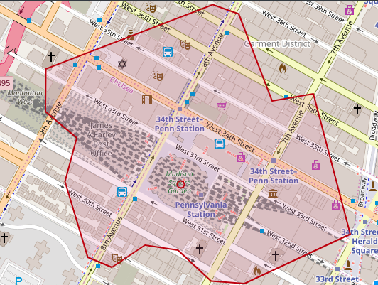
As we are handling real NYC Yellow Taxi trip data, let’s imagine several queries that could represent a real evaluation. We selected several famous places in NYC and, thanks to MapBox Open API, we obtained the geometry representation of:

• 5-minute walking area from Madison Square Garden.
• 5-minute walking area from New York Yankees Stadium.
• 5-minute walking area from Wall Street.
• 5-minute area walking from Broadway.

To provide an idea of the range of these areas, the following shows about how a 5-minute walking isochrone appears (using as an example the 5- minutes walking area from Madison Square Garden):

Having these isochrones, we thought it would be useful for a taxi business to know, for example:

1. Taxi passenger pick-ups during 2013, within a 5-minute walking area from Madison Square Garden.
2. Taxi passenger pick-ups during 2013, within a 5-minute walking area from New York Yankees Stadium.
3. Hourly report of taxi passenger pick-ups within a 5-minute walking area from Wall Street. 
4. Daily report of taxi passenger pick-ups within a 5-minute walking area from Broadway. 

QUERY 1: TAXI PASSENGER PICK-UPS DURING 2013 JANUARY, FEBRUARY, AND MARCH WITHIN A 5-MINUTE WALKING AREA FROM MADISON SQUARE GARDEN.

LeanXcale query 1:

SELECT count(*) FROM trip_data WHERE 
ST_Intersects( 
ST_GeomFromText('POLYGON ((-73.992462 40.754578,-73.991676
40.754368,-73.990669 40.752377,-73.989418 40.752537,-73.988304
40.749332,-73.991508 40.748196,-73.992516 40.74826,-73.993507
40.748962,-73.994507 40.749081,-73.995506 40.748577,-73.996231
40.748802,-73.996925 40.750534,-73.996567 40.751534,-73.997513
40.752136,-73.997505 40.753113,-73.992462 40.754578))'),
ST_MakePoint(pickup_longitude,pickup_latitude));

PostgreSQL query 1:

select count(*) FROM trip_data WHERE 
ST_Intersects(
ST_GeomFromText('POLYGON ((-73.992462 40.754578,-73.991676
40.754368,-73.990669 40.752377,-73.989418 40.752537,-73.988304
40.749332,-73.991508 40.748196,-73.992516 40.74826,-73.993507
40.748962,-73.994507 40.749081,-73.995506 40.748577,-73.996231
40.748802,-73.996925 40.750534,-73.996567 40.751534,-73.997513
40.752136,-73.997505 40.753113,-73.992462 40.754578))',4326),
geom_pickup)

QUERY 2: TAXI PASSENGER PICK-UPS DURING 2013 JANUARY, FEBRUARY, AND MARCH WITHIN A 5-MINUTE WALKING AREA FROM NEW YORK YANKEES STADIUM. 

(In the following queries, only the area representation changes as these are the same queries in the previous case).

LeanXcale query 2:

SELECT count(*) FROM trip_data WHERE 
ST_Intersects (
ST_GeomFromText('POLYGON ((-73.922783 40.833035,-73.921013
40.829689,-73.923134 40.82869,-73.9226 40.828205,-73.9226
40.826694,-73.927124 40.825451,-73.927444 40.826691,-73.928711
40.82769,-73.928688 40.829258,-73.927124 40.829372,-73.926949
40.829861,-73.927643 40.830688,-73.927177 40.831741,-73.926125
40.83247,-73.925125 40.832592,-73.924126 40.833294,-73.922783
40.833035))'), 
ST_MakePoint(pickup_longitude,pickup_latitude))

PostgreSQL query 2:

SELECT count(*) FROM trip_data WHERE 
ST_Intersects (
ST_GeomFromText('POLYGON ((-73.922783 40.833035,-73.921013
40.829689,-73.923134 40.82869,-73.9226 40.828205,-73.9226
40.826694,-73.927124 40.825451,-73.927444 40.826691,-73.928711
40.82769,-73.928688 40.829258,-73.927124 40.829372,-73.926949
40.829861,-73.927643 40.830688,-73.927177 40.831741,-73.926125
40.83247,-73.925125 40.832592,-73.924126 40.833294,-73.922783
40.833035))',4326), 
geom_pickup)

QUERY 3: HOURLY REPORT OF TAXI PASSENGER PICK-UPS WITHIN A 5-MINUTE WALKING AREA FROM WALL STREET DURING 2013 JANUARY, FEBRUARY, AND MARCH.

LeanXcale query 3:

select hour(floor(pickup_datetime to hour)) as hourtime, count(*) as total from trip_data WHERE 
ST_Intersects (
ST_GeomFromText('POLYGON((-74.005943 40.710003,-74.00499
40.706955,-74.005058 40.704586,-74.006203 40.703728,-74.008728
40.703255,-74.010208 40.703156,-74.012238 40.703709,-74.013412
40.706734,-74.013306 40.707733,-74.012054 40.709583,-74.009209
40.710201,-74.005943 40.710003))'), ST_MakePoint(pickup_longitude,pickup_latitude)) 
group by hour(floor(pickup_datetime to hour))

PostgreSQL query 3:

select extract(hour from pickup_datetime) as hourtime, count(*) as total from trip_data WHERE 
ST_Intersects (
ST_GeomFromText('POLYGON((-74.005943 40.710003,-74.00499
40.706955,-74.005058 40.704586,-74.006203 40.703728,-74.008728
40.703255,-74.010208 40.703156,-74.012238 40.703709,-74.013412
40.706734,-74.013306 40.707733,-74.012054 40.709583,-74.009209
40.710201,-74.005943 40.710003))',4326), 
geom_pickup) 
group by extract(hour from pickup_datetime)

QUERY 4: DAILY REPORT OF TAXI PASSENGER PICK-UPS WITHIN A 5-MINUTE WALKING AREA FROM BROADWAY, DURING 2013 JANUARY, FEBRUARY, AND MARCH.

LeanXcale query 4:

SELECT dayofweek(floor(pickup_datetime to day)) as pickupday, 
count(*) as total from trip_data WHERE ST_Intersects(
ST_GeomFromText('POLYGON((-73.982025 40.761963, -73.980431
40.757938,-73.980927 40.756939,-73.983986 40.755882,-73.987045
40.755211,-73.987541 40.755432,-73.989449 40.759937,-73.988937
40.760941,-73.988037 40.761616,-73.984047 40.762516,-73.983047
40.762589,-73.982025 40.761963))'), ST_MakePoint(pickup_longitude,pickup_latitude))
group by dayofweek(floor(pickup_datetime to day))

PostgreSQL query 4;

select extract (dow from pickup_datetime) as pickupday, count(*) as total from trip_data WHERE 
ST_Intersects(
ST_GeomFromText('POLYGON((-73.982025 40.761963, -73.980431
40.757938,-73.980927 40.756939,-73.983986 40.755882,-73.987045
40.755211,-73.987541 40.755432,-73.989449 40.759937,-73.988937
40.760941,-73.988037 40.761616,-73.984047 40.762516,-73.983047
40.762589,-73.982025 40.761963))',4326), 
geom_pickup) 
group by extract (dow from pickup_datetime)

SCENARIOS

For this benchmark, we cover tests for the following cases:

1. trip_data table storing information about NYC Yellow Taxi trips during 2013 for January, February, and March (~40 million rows).
2. The complete NYC Taxi trips dataset, during 2013, from January to December (~165 million rows).

Query executions are performed with DBeaver as a general database JDBC client.

SCENARIO 1

With the trip_data table storing ~40 million rows.

Results:

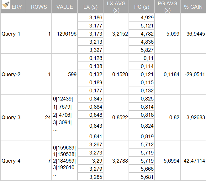
Given these results, we consider this scenario contains 40 million rows, and the LeanXcale and PostgreSQL performances are quite close. LeanXcale appears a little better for query 1 and query 4, and PostgreSQL appears a little better for query 2 and query 3. The cases in which PostgreSQL is better means a difference of milliseconds, while the cases in which LeanXcale is better brings a difference of 2 seconds, as in the case of query 4.

What if we load the entire 2013 dataset on both databases?

SCENARIO 2

With the trip_data table storing ~165 million rows.

Results:

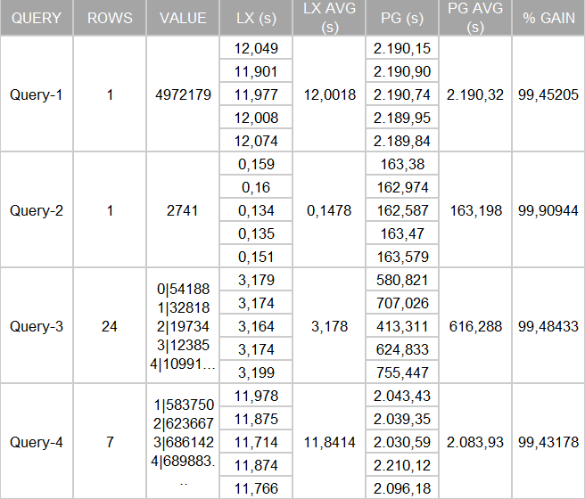
We can see the results speak for themselves. There’s a gain of 99% on the query timing for searches over the geographical columns by LeanXcale. We also executed the queries over the PostgreSQL read replica with similar timings returned. 

Next, we performed a vertical scaling on PostgreSQL. So, we created a new scenario where the physical AWS machine was improved to an “m5.4xlarge” AWS RDS service featuring 16 virtual cores, 64GB of RAM, and 300 GB of disk. We also created a read replica.

SCENARIO 3

With the trip_data table storing ~165 million rows and multiplying the PostgreSQL machine power by 4.

Results:

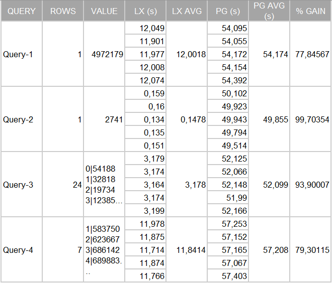
Given these new results, the PostgreSQL times are better compared to the previous configuration, which is expected. However, this level of performance remains far from the performance offered by LeanXcale. 

This significantly enhanced performance occurs thanks to the GIS filtering geohash-based algorithm developed by LeanXcale that takes advantage of the great performance of the Kivi Data Store offers. You can learn more from our whitepapers.

CONCLUSION

LeanXcale is a fully distributed database that provides outstanding performance for any size. The larger the dataset, the better the speed difference. With a moderate size database (40 million rows), LeanXcale is around 40% faster for heavy queries. With 165 million rows, the difference increases up to 99%, which is a difference that cannot be reduced even after scaling-up the PostgreSQL instance.

LeanXcale’s behavior is based on the combination of three components: its data-store efficiency, its scalable architecture and its Geo-has algorithm implementation. LeanXcale is the perfect alternative, since maintain when other GIS solutions cannot deal with the volumes.

Sponsored by LEANXCALE