How to choose a predictive algorithm.
How to choose a predictive algorithm.
By MICHAEL BOWLES.
You have to build a system for making predictions (which customers are going to leave, what ad will get clicked, which claims are fraudulent) based on what you know now (how much has the customer been using your app, what have they clicked in the past, what is their claim history). How do you attack the problem? There are several steps that you’d inevitably take – get a feel for the data, choose a few algorithms and evaluate their performance. This article will discuss how you might choose the algorithms to try out on your problem. The basic line of reasoning and the examples come from Chapter 3 in Machine Learning in Python: Essential Techniques for Predictive Analysis. All of the material from the book is used with permission of Wiley, the publisher.
The first thing is to be clear about the nature of the predictive problem. Table 1 below, gives a simple illustration.
| Outcomes | Feature1 | Feature2 | Feature3 |
| Clicked on Link | Gender | $ Spent on Site | Age |
| Yes | M | 0.0 | 25 |
| No | F | 250 | 32 |
| Yes | F | 12 | 17 |
Table 1: Simple Example of Predictive Problem
Each row of data in the table corresponds to a visit to a website. The first column records the visitors response to link presented to them. Did the visitor click the link or not. The other columns give other facts about the customer – demographic data like gender and age and how much they spent on the site. The basic prediction problem is determine whether or not future customers will click on a link. This data is in a form that is called “structured data”. Structured data is data that can be arranged in the rows and columns of a table. A table you might build from a database provides a familiar example.
The data in the table comes in two flavors. One column represents the thing you’re trying to predict and the other columns are what you have available to predict it. These two types of data each go by several names which can make it confusing to read the literature until you become familiar with the variations. The thing you’re trying to predict is variously called outcome, end point, target or label. The things you can base the prediction on are called predictors, features, regressors, variables or attributes. It’s not unusual to have these variables change roles in order to make predictions for different business purposes. For example instead of predicting whether the visitor will click on the link, you might wish to predict how much they will spend on the site and you might (or might not) use clicking on the link as an input to the prediction. Those kinds of choices depend on business needs and operational reality of what things are available at the point of needing the prediction. Unstructured data do not fit into the form of a table. Free form text, images and spoken voice are examples of unstructured data.
Some algorithms are better suited to structured data and some are better suited to unstructured problems. My friend Anthony Goldbloom, CEO and founder of Kaggle (Kaggle.com) shared his views with me. Kaggle.com organizes hundreds of machine learning competitions to help corporations around the world get a leg up on their predictive problems. That gives Anthony good perspective of what delivers the best performance. He told me that the machine learning algorithms used by contest winners depend on the nature of the problem. For structured problem the winners most likely use ensembles of binary decision trees and spend most of their energy manipulating the features, whereas for unstructured problems the best performers use deep neural nets and spend their time determining the shape of the neural net. The algorithms covered in Machine Learning in Python are well suited to structured problems and you’ve made your first algorithm decision. If your data are structured use an algorithm appropriate to structured data. Next you see how the amount of data you have and the complexity of your problem can help you understand what structured algorithm will give the best performance. Anthony’s choice of tree ensembles will be one of the candidates, but you’ll see that there are cases when you’ll make a different choice.
One of the factors in your choice of algorithm is the complexity of your problem. Figure 1 gives an illustration of a simple classification problem. That figure will help explain what is meant by a simple problem. Figure 1 plots examples such as those from Table 1. Each point represents a single experiment The two axes in the figure correspond to the values of two attributes. In the figure those attributes are real-values number like “Age” and “$ Spent on Site” from Table 1. The color of the points indicates the value of the binary label for that point. These correspond to a label like the click, no-click labels in Table 1.
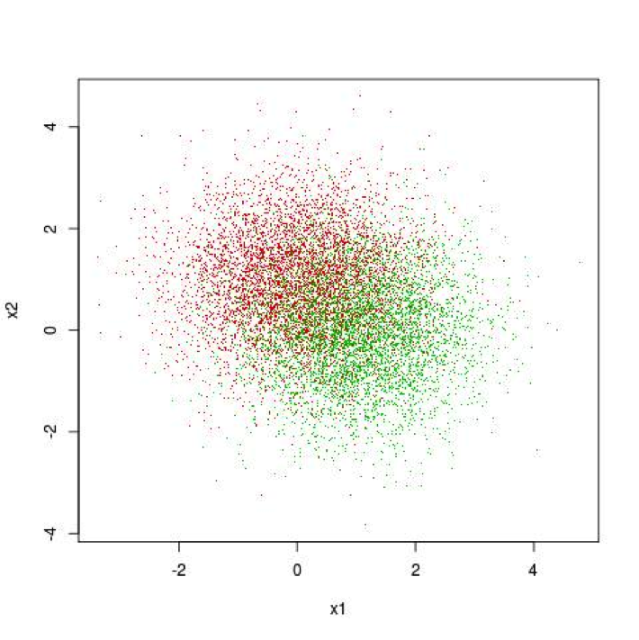
Figure 1. Illustration of a Simple Classification Problem
The problem of building a predictive model for Figure 1 is to draw a curve in the x1, x2 plane. Given this curve the prediction model is straightforward. Points on one side of the curve will be predicted to have the label of the green and points on the other side as the label of the red points. There’s a portion in the middle of figure where green and red points are interspersed amongst one another. No model can separate those perfectly. The best curve separates the red points from the green points in some statistical sense – like average misclassification error. What makes the problem of Figure 1 a simple problem is that the best curve for this problem is a very simple curve – a straight line. Figure 2 adds the best predictive (separating line) to the points shown in Figure 1. The line in Figure 2 was constructed using a penalized logistic regression package available in Python scikit-learn.

Figure 2. Simple Classification Problem with Best Separating Curve Added
By contrast to the simple problem shown in Figures 1 and 2, Figure 3 shows a more complicated problem. Notice that there appear to be islands of red dots in the upper right hand corner of the plot. It seems more or less clear that a more complicated curve might be able to out-perform a straight line on this problem. You might imagine tracing such a line in your mind’s eye and giving the line crenulations and peninsulas to include areas where one color visibly out-numbers the other.
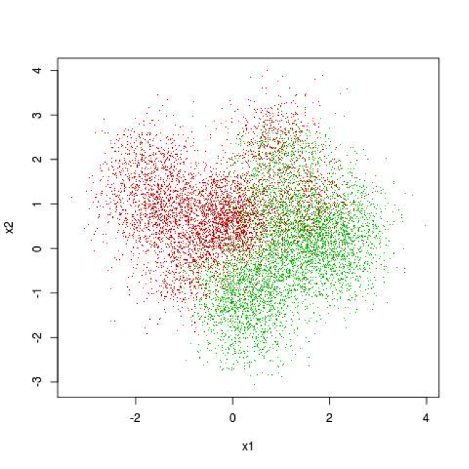
Figure 3. Illustration of a Complicated Classification Problem
Figure 4 depicts a separating curve for the data in Figure 3. The curve depicted in Figure 4 was built using one of the tree ensemble packages available in scikit-learn. The curve probably follows some of the contours that you envision as you imagine the shape of the curve while looking at the raw data. But the curve also has a glitch in the upper right hand corner.
Ensemble tree methods build complicated models that are required to accurately model complicated problems.
They are capable producing high-fidelity models replicating very fine-grained detail of things like customer behavior, but they require a lot of data to build. More data would probably remove the glitch in the upper right hand corner of Figure 3.
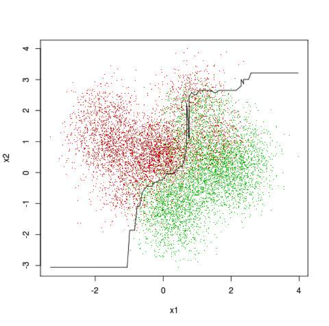
Figure 4. Complicated Classification Problem with Separating Curve Derived with scikit-learn Tree Ensemble Package
These examples illustrate why there’s so much excitement surrounding big data. Large data sets can support building finely detailed models of complicated problems. On the other hand, if the problem is simple, as in the Figures 1 and 2, then a simple model can get the same performance as a complicated one. What about if the data isn’t big?
Discussion of bigness in data frequently glosses over some important distinctions. Consider the simple dataset in Table 1.
That dataset could grow to be big by adding more rows or by adding more columns (or by doing both). That difference is important for fitting a model. Adding more rows means adding more points to Figures 1 – 4, for example. Adding more columns would mean adding more dimensions to those figures. When you don’t have many examples, adding more facts about them may make it harder to fit a complicated model. As an extreme example suppose that you’ve got genomic data on two persons.
You’ve got millions of facts about each one, but too little to isolate the source of a genetic disorder that one may have.
Many millions of base pairs may be different between them. Adding more data isn’t going to help. So in cases where the data table has relatively many columns (attributes) compared to the number of rows (examples) you may get better performance from a simpler linear method than you do from a more complicated ensemble method.
Figures 5 and 6 respectively show the same basic data set as in Figures 1 – 4, but with many fewer data points. Figure 5 shows a penalized logistic regression line fit to the data and Figure 6 shows an ensemble tree model fit to the data.
These are analogous to Figures 2 and 4. Figure 5 shows a straight line slanting from lower left to upper right.
Figure 6 shows basically a step-wise function that roughly approximates the straight line in Figure 5. They deliver fairly close performance to one another.
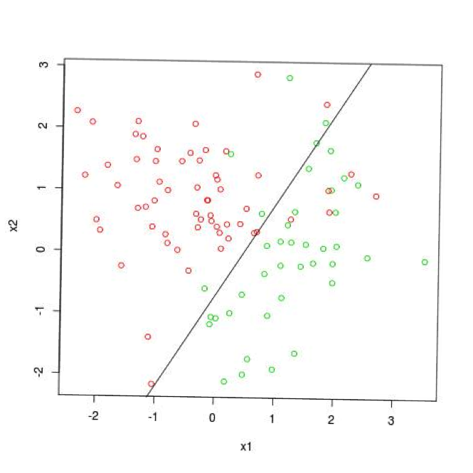
Figure 5: Simple Model Fit to Complicated Problem with Too Little Data for Complex Model
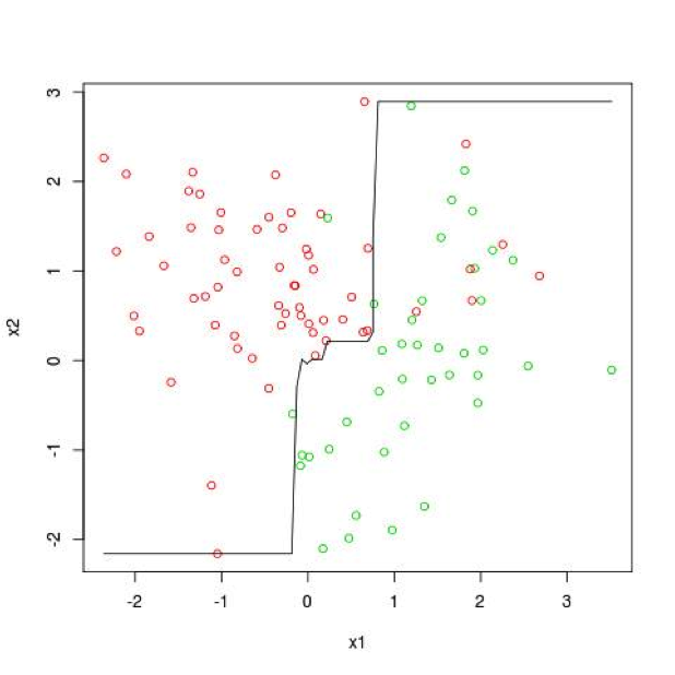
Figure 6: Complex Model Fit to Complicated Problem with Too Little Data for Complex Model
Summary and Other Considerations
This article has addressed the question of what algorithm you should use for building predictive models. The article has outlined several features of the problem that might guide your selection. Those include the complexity of the problem, the number of rows and columns of data in your data set and whether your problem is structured or unstructured.
The tradeoffs covered here have been primarily in terms of optimizing prediction performance. Several other aspects of your problem setting might influence your choices. For example training times or evaluation times for complicated models may drive you to choose a linear model. High frequency traders, for example need to generate predictions in microseconds or less. It can be difficult to generate a prediction with an ensemble of tree model in that little time.
For structured problems where the data can be arranged in a table like those that can be built from databases comparisons have been shown to illustrate how problem complexity and the number of rows versus columns (examples versus attributes) might drive your choice between a linear algorithm like penalized regression of an ensemble of trees (gradient boosting, random forests and hybrids).
Resources
Book: Machine Learning in Python: Essential Techniques for Predictive Analysis. Michael Bowles. Wiley, ISBN: 978-1-118-96174-2, 360 pages May 2015